


Taxicabs in Chicago form a vital part of the city’s transportation network. The industry’s growth and sustainability heavily depend on enhancing customer services and transparency. An aspect that customers often value is the ability to anticipate and predict the costs of their trips in advance. This blog explores how machine learning techniques can transform taxi services, by leveraging datasets on Chicago Taxi Trips and utilizing Google Cloud services.
Unleash The Power Of Machine Learning With Niveus
Business Goal: Driving towards a Customer-centric Future with Predictable Pricing
The industry is striving to enhance customer experience through transparent fares, empowering riders and boosting operational efficiency, ultimately aiming for sustainable growth. By introducing predictable pricing, Chicago’s taxis aim to build trust, optimize costs, and adapt to market demands, all in pursuit of a thriving and customer-centric future.
Navigate to Smarter Fares and Smooth Rides
Taxicabs in Chicago are operated by private companies and licensed by the city, with about seven thousand licensed cabs operating within the city limits. The industry is looking to elevate customer experiences by providing transparent and predictable fare estimates with the aim to improve the quality of services provided. Anticipating trip costs in advance allows customers to make informed decisions, fostering trust and aiding increased choice between solo rides and carpooling.
Further, accurately predicting trip totals in advance will lead to optimized pricing strategies, improved customer relationships, operational efficiency, and better market adaptability, all of which in turn are crucial for the growth and sustainability of taxi services.
Leveraging Machine Learning Models for Precision and Accuracy
The Chicago Taxi Trips dataset, with its massive scale and complexity, necessitates a machine learning approach. Traditional methods struggle to handle such vast datasets effectively. Machine Learning Solutions offer predictive models trained on historical trip data, enabling precise fare predictions. Chicago Taxi Trips dataset includes data on trips spanning from 2013 to the present, and has 23 columns, approximately 200 million rows, and is about 75 GB in size.
How the Machine Learning Models Addresses the Business Goal
Machine Learning supports a variety of predictive models. Depending upon the complexity of the problem, the right model can be built to predict the trip fare. Predictive models will be trained on available data. After performing required analysis, models will be then tuned and tested for accuracy. Machine Learning models allow scaling, complex data analysis, training over new data, real time predictions, and building complex pipelines to manage and streamline business processes. Accurate predictions will help taxi companies in making dynamic pricing adjustments based on various factors like demand, time of day, and trip distance. This will not only maximize revenue opportunities but also ensures competitive pricing, helping taxi companies to stay viable in the market. Moreover, this approach allows for more strategic resource allocation, such as deploying taxis to high-demand areas, thereby enhancing operational efficiency and customer satisfaction.
Understanding the Data Landscape: A Glimpse into Fare Trends and Customer Behavior
Here, we take a deep dive into the various types of data exploration used to uncover hidden patterns and trends within the data. Let’s examine how descriptive statistics, trend analysis, comparisons, and even hypothesis formation work together to paint a comprehensive picture of the market landscape. By delving into these different facets of exploration, we gain valuable insights that inform our understanding of customer behavior, pricing strategies, and the overall dynamics of the transportation sector.
Types of Data Exploration Performed
The data exploration performed can be categorized into several types:
- Descriptive statistics: This involves summarizing the data using measures like mean, median, mode, and standard deviation. The text mentions that “the rise in average fares is significant” and “the highest payment counts are for credit cards and cash,” which are both examples of descriptive statistics.

Code Image 1: Average Fare for each hour of every day over the week post the pandemic
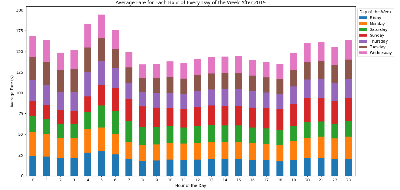
Figure 1: Average Fare for each hour of every day over the week post the pandemic
- Trends Analysis: This involves identifying trends and patterns in the data over time. The text mentions that “2023 saw a sharp decrease in trip counts” and “the dominance of Taxi Affiliation Services,” which are both examples of trends and patterns.
Code Image 2.1: Trend of Average Trip Total post pandemic
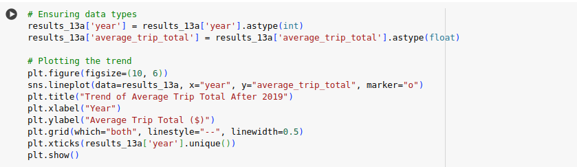
Code Image 2.2: Trend of Average Trip Total post pandemic
Figure 2: Trend of Average Trip Total post pandemic
- Comparisons: This involves comparing different groups or categories of data. The text mentions that “with increasing taxi fares, customers might compare these costs with alternatives” and “higher prices may deter customers, especially if alternative transportation options are more affordable,” which are both examples of comparisons.
Code Image 3: Total Revenue Generated by Individual taxi companies post pandemic
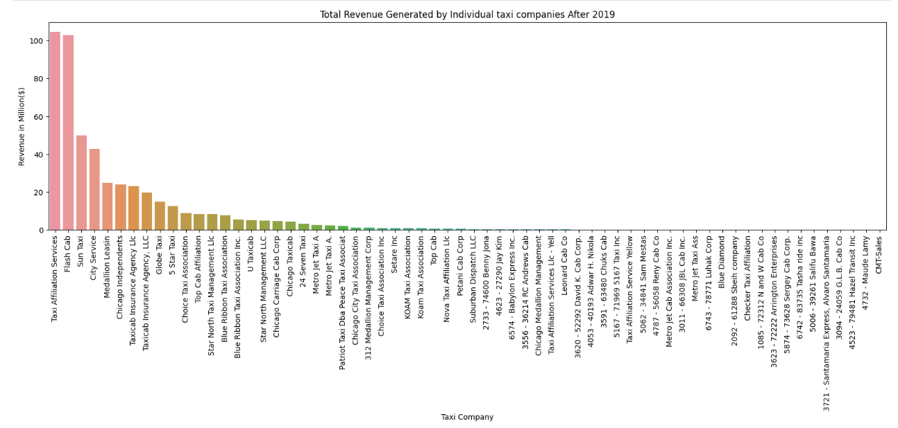
Figure 3: Total Revenue Generated by Individual taxi companies post pandemic
- Hypotheses: This involves developing hypotheses about the relationships between different variables in the data. The text mentions “the need for a dynamic and adaptive pricing strategy becomes even more crucial” and “This situation, considered alongside the increased average fares and customer churn, suggests a rapidly changing market landscape,” which are both examples of hypotheses.
The Decisions Influenced by Data Exploration
The data exploration in the passage influenced several decisions, particularly in three key areas:
Pricing Strategy:
- High average fares and customer churn: Data showed a significant rise in average fares and a corresponding drop in customer numbers. This suggested that prices might be too high and driving customers away. This insight influenced the decision to consider adopting a dynamic and adaptive pricing strategy that could adjust fares based on demand and competitive landscape.
- Comparison with alternatives: Data exploration highlighted the potential customers were comparing taxi fares with more affordable options like ride-sharing and public transport. This insight influenced the decision to re-evaluate current pricing and consider strategies to make taxis more competitive.
Payment Options:
- Popularity of credit cards and cash: Data showed that credit cards and cash were the most preferred payment methods. However, the popularity of mobile payments, particularly among tech-savvy customers, was also noted. This insight influenced the decision to expand payment options and integrate advanced digital payment solutions to attract a wider range of customers.
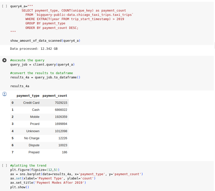
Code Image 4: Payment Modes post pandemic
Figure 4: Payment Modes post pandemic
Market Trends:
- Declining trip counts and market consolidation: Data revealed a sharp decrease in overall taxi trips and the closure of numerous companies. This suggested a rapidly changing market with shrinking demand or significant challenges. This insight influenced the decision to become more aware of market trends and adapt operations accordingly to remain competitive.
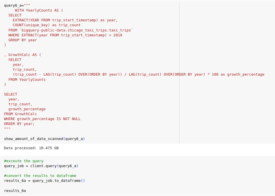
Code Image 5.1: Yearly Trip counts and Growth Percentage post pandemic
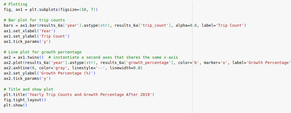
Code Image 5.2: Yearly Trip counts and Growth Percentage post pandemic
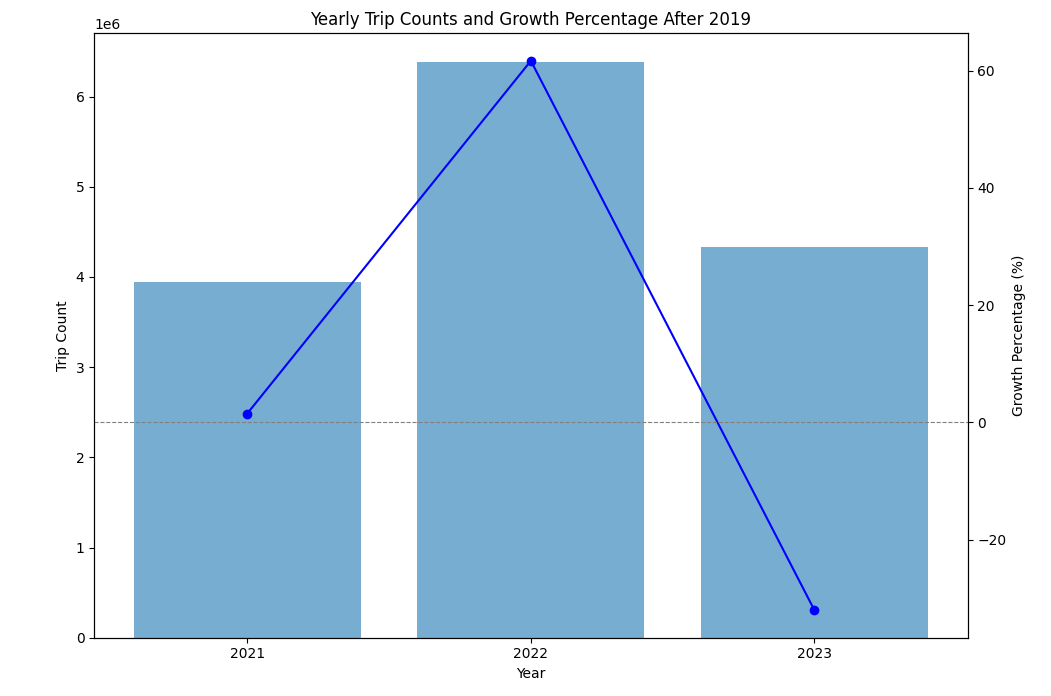
Figure 5: Yearly Trip counts and Growth Percentage post pandemic
Feature Engineering: Refining the Data for Accurate Fare Prediction
This section delves into the feature engineering process performed to optimize the dataset for accurate trip fare prediction. The focus is on eliminating redundant information while retaining crucial features that significantly impact trip cost.
Types of Feature Engineering Performed:
The feature engineering processes that were performed were of several types. These include:
- Reduced redundant columns:
While trip details like time and location were dropped, retaining relevant, non-redundant information from comparable columns offers a streamlined dataset with focused insights.
- No direct correlation with pickup/dropoff coordinates:Initial analysis indicated that coordinates alone are insufficient for predicting trip_total.
- Incorporated community area identifiers: Included due to their significant influence on trip_total variations and enhanced model accuracy by considering geographical fare differences.
- Aggregated data by community areas: Highlighted the necessity of area-based analysis for accurate fare prediction. Showed that community areas impact fares at both trip origins and destinations. The consistent impact across locations emphasizes their importance in the model. Essential for precise trip_total predictions. Helps align the predictive model with actual fare structures.
- Non-linear relationship identified: Community areas and trip_total exhibit a complex, non-linear relationship. Suggests the need for advanced modeling techniques to capture this dynamic.
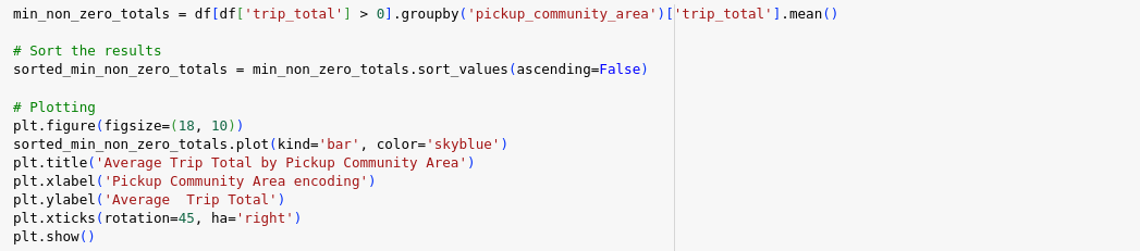
Code Image 6: Average Trip Total Pickup Community Area

Figure 6: Average Trip Total Pickup Community Area
The Features Selected for the Model and Why.
As feature selection plays a vital role in building suitable and efficient algorithms, below are some feature selection operations performed:
- Removed pickup_census_tract and dropoff_census_tract: Eliminated due to high levels of missing data (around 60% null values). Their absence helps streamline the dataset for more efficient analysis.
- Dropped unique_key and taxi_id: Identified as non-contributory to the model, adding no predictive value. Removal focuses the model on more impactful variables.
- Excluded components (fare, tips, tolls, extras): Found strong correlation with trip_total, risking multicollinearity.
Their exclusion avoids potential model bias and overfitting.
Code Image 7: Model Feature Selection using HeatMap

Figure 6: Model Feature Selection
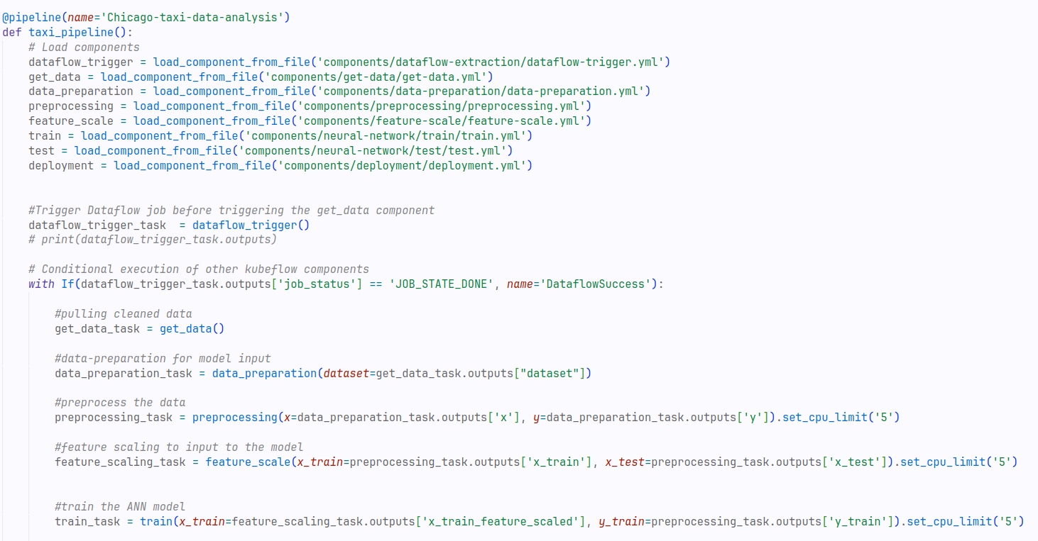
Pre-processing and the Data Pipeline:
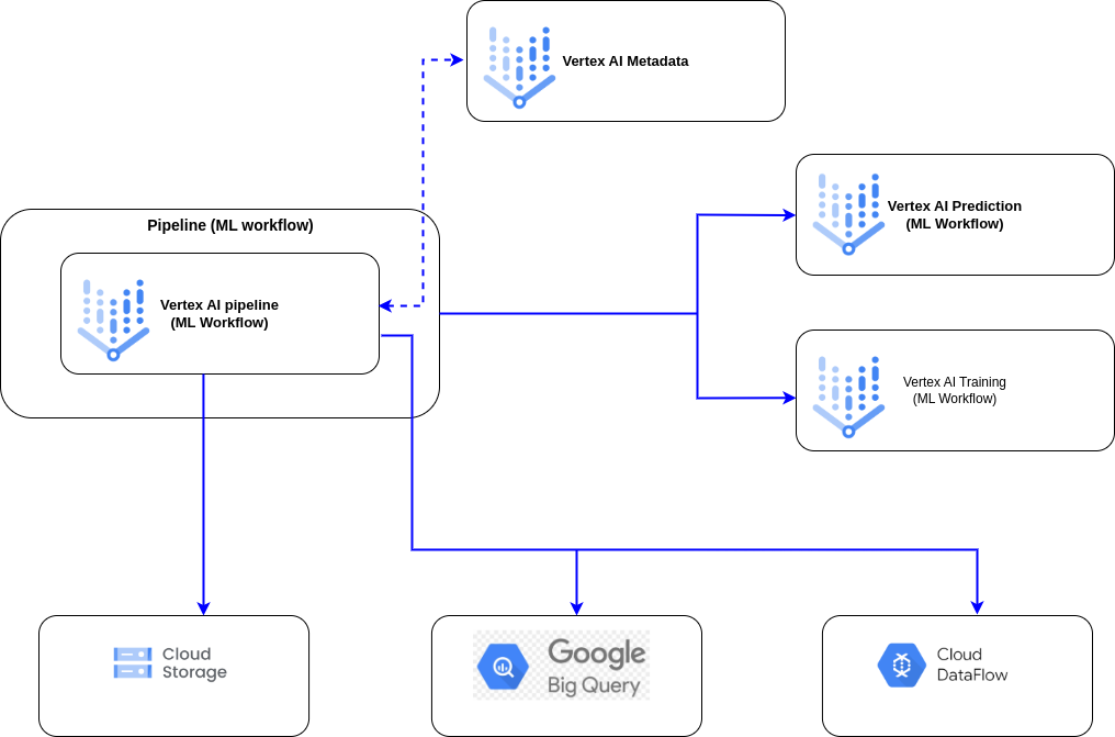
Figure 7: High level GCP Architecture
Data from the source system was loaded into the Cloud Storage bucket, where data files were stored. Dataflow was then used to load data from Cloud Storage to BigQuery. During the first load, all the data was loaded, and in subsequent loads, only delta data was loaded from the source. All pre-processing steps were done to load clean data into BigQuery. This data fetching from the source system and performing a pre-processing step was exposed to an API endpoint using Cloud Run, and the data could be consumed from this callable API endpoint.
Data available from the above API endpoint could then be consumed for building the ML model in Vertex AI. For notebooks, Vertex AI user-managed notebooks were used to get more controlled and optimized performance. Model development, training, and testing were done in Vertex AI.
After the model was developed and tested, the code was then Dockerized, and Docker images were created. These Docker images were then used to create an end-to-end machine learning pipeline. Once the pipeline was developed, it was deployed on Vertex AI pipelines. Vertex AI pipelines allowed running the entire machine pipeline to train the model on the latest data in a controlled and efficient manner.
Prediction models were exposed to endpoints to cater to users/systems and provide predictions in real-time. Vertex AI model registry was used to organize, track, and deploy models.
Machine Learning Model Design(s) and Selection:
Machine learning model design and selection played a crucial role in the overall ML pipeline. This involved training multiple models with different configurations and comparing their performance on metrics relevant to the specific problem. Ultimately, the chosen model struck a balance between performance, complexity, and other practical considerations, yielding valuable insights from the data.
The Model/Algorithm(s) Chosen
Based upon the analysis performed, an Artificial Neural Network (ANN) built with Keras emerged as the best choice for tackling this specific ML problem.
The Criteria for Machine Learning Model Selection
Here are the criteria used for machine learning model selection:
ANN – Artificial Neural Network
- Capturing non-linear Relationships – ANNs excel at modeling the non-linear dynamics between community areas and trip_total.
- High-dimensional Data Handling – ANNs effectively manage datasets with numerous features, outperforming traditional models in high-dimensional spaces.
- Flexibility and Adaptability – The adjustable architecture of ANNs allows for dataset-specific optimization, surpassing the rigidity of models like XGBoost.
- Feature Interactions – ANNs automatically detect and utilize interactions between key variables such as time, location, and distance for trip_total prediction.
- Robustness to Overfitting – Techniques like dropout and weight regularization make ANNs less prone to overfitting, ensuring better generalization to new data.
- Scalability – ANNs scale efficiently with increasing data volume and complexity, a crucial aspect for evolving datasets like taxi trip records.
- Performance with Complex Data – ANNs seamlessly handle diverse data types, including both numerical and categorical data, without extensive preprocessing.
- Continuous Learning and Improvement – ANNs’ capacity for online learning enables them to adapt and improve as new data emerges, advantageous in dynamic environments.
Keras
- User-Friendly Interface – Keras offers a straightforward interface for building and experimenting with various neural network architectures.
- Hyperparameter Customization – Easily customize hyperparameters such as layers, neurons, activation functions, and learning rates to find the optimal model configuration.
- Documentation Support – Keras provides concise and well-structured documentation, aiding users in understanding and selecting the most suitable models.
- Handling Large Datasets – Keras is designed to handle massive datasets efficiently, making it suitable for applications with extensive data.
- Capturing Complex Relations – Keras excels at capturing complex relationships within data, making it ideal for tasks where intricate patterns and dependencies exist.

Code Image 8: Model Configuration and Parameters
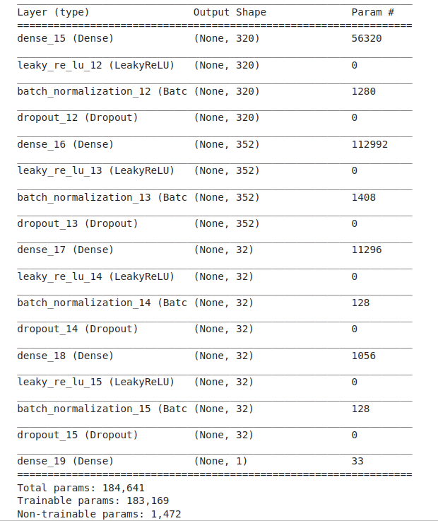
Figure 8: Model Configuration and Parameters
Machine Learning Model Training and Development
- The dataflow-preprocessing was also deployed to a cloud endpoint, which could be consumed as a callable API. This provided clean data from tables.
- Then the cleaned data was pulled from BigQuery for data preparation.
- The data was split into selected features chosen after EDA and target variables for model training.
- Further, the data was treated for outliers and null imputation. Additionally, the feature variables underwent preprocessing.
- In the preprocessing step, column transformation using one-hot encoding was performed. Lastly, the data was split into train and test datasets.
- For feature scaling, standardization was performed using StandardScaler.
- This processed dataset was used for training the ANN model.
- The model was then saved to the model registry for endpoint deployment for online prediction and for batch predictions.
- The batch predictions were saved to the GCS as test component artifacts.
Code Image 9: VertexAI MLOps Pipeline 

Figure 9: VertexAI MLOps Pipeline
Dataset Sampling Used for Model Training
Following the completion of the Exploratory Data Analysis (EDA), the insights gleaned illuminated a noticeable decline in taxi bookings, accompanied by a downturn in both trip frequency and revenue. The data also revealed the unfortunate shutdown of multiple taxi companies post-2020. Given that the demo was prepared in 2023, the dataset is now employed to forecast the total number of trips for the year 2023. This predictive analysis aims to provide valuable foresight into the taxi industry’s trajectory, facilitating informed decision-making and strategic planning for the year ahead.
Google Cloud Best Practices for Distribution, Device Usage and Monitoring
The model training process utilized a custom training pipeline within Vertex AI to train an Artificial Neural Network (ANN) model. Optimizing for device utilization, an e2 machine (a machine type optimized for memory-intensive workloads) was selected. Scalability was further achieved by scaling by adding more machines of the same type, increasing the training module’s capacity. Notably, this training scenario did not involve GPU usage. This strategic resource utilization enhances efficiency and ensures the effective training of the ANN model for the specified task.
Optimal Model Evaluation Metric Aligned with Business Goals
In evaluating the performance of the Artificial Neural Network (ANN) model, the R-squared (R2) value was chosen as the accuracy parameter. Both the training and test datasets were assessed based on this parameter, with the goal of minimizing the R2 score. By doing so, we aimed to minimize prediction errors in the trip total, ensuring that the ANN model provides robust and accurate forecasts for the task at hand.
Train dataset | Mean Absolute Error | 3.622 |
| Root Mean Absolute Error | 6.850 | |
Test dataset | Mean Absolute Error | 3.18 |
| Root Mean Absolute Error | 6.39 | |
| Accuracy(R-squared) | 91.22% | |
Table 1: Performance Evaluation
Hyperparameter Tuning and Model Performance Optimization
- Stagnation Observation – Identified a stagnation phase in Mean Squared Error (MSE) improvement, indicating a potential plateau in learning.
- Epoch Reduction – Decreased the number of epochs to 20 epochs to streamline training duration while optimizing time efficiency.
- Batch Size Increase – Augmented batch size to 1732 for more impactful weight updates, ensuring substantial progress even with fewer epochs.
- Increased Dataset – Simultaneously increased the number of data points, maintaining the quality of training batches despite fewer epochs (The current data points are 55 lakhs records).
- Keras Tuner – Keras tuner was used for selecting the hyperparameters such as number hidden layers and its units, dropout rates , input layer units and learning rate. It auto selects the best params by trying and iterating several different parameter combinations.
- These were the best chosen parameters by the keras tuner.
{‘units_input’: 320, ‘dropout_input’: 0.2, ‘num_layers’: 3, ‘units_0’: 352, ‘dropout_0’: 0.4, ‘learning_rate’: 0.0007090582191927241, ‘units_1’: 32, ‘dropout_1’: 0.2, ‘units_2’: 32, ‘dropout_2’: 0.2}
| Parameters | Obtained value |
| Number of Epoch | 20 |
| Batch Size | 1732 |
| Dataset count | 55 lakh record |
| Learning rate | 0.0007090582191927241 |
Table 2: Parameters chosen for Model fit
Determining Variances and Optimizing ML Model Architecture
To avoid overfitting, we implemented three strategies. First, we reduced the training epochs to 20, which helps prevent the model from memorizing noise in the training data. We also increased the batch size to 1732, encouraging more generalized learning. Second, we expanded the dataset to 55 lakh records, allowing the model to learn from a broader range of data and capture more complex patterns, mitigating underfitting. Finally, we utilized Keras Tuner for hyperparameter optimization, striking a balance between model complexity and regularization. This directly addressed the bias-variance trade-off by fine-tuning the network’s depth and learning capacity.
Machine Learning Model Evaluation
- Online prediction helps in providing predictions to the real-time data that would be helpful for timely made decisions.
- The Vertex AI pipeline does a model deployment to be consumed for real time predictions.
- Steps for real time predictions are:
- We create a request.py in picking up the inputs from the UI screen.
- Within this the column Transform and standard scaler pickle files are used that would help in converting and standardizing the input values to be suitable for the model input.
- This script can be directly executed in the cloud shell, to get the real-time predictions.

Figure 10: Real Time Prediction Results
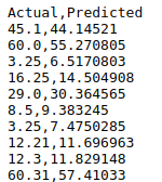
Figure 11: Batch Prediction Results
Conclusion:
This exploration of applying machine learning and MLOps to the Chicago taxi industry serves as a powerful microcosm for the broader impact these technologies are destined to have on every corner of the business world. We’ve witnessed how data, once inert numbers, can be transformed into a potent force for change. By anticipating needs and preferences, ML personalized offerings build trust and fosters loyalty, paving the way for thriving customer-centric businesses. The Chicago taxi industry is just one example of the vast potential unleashed by ML and MLOps. From healthcare to finance, and retail to manufacturing, every industry stands to benefit from the transformative power of these technologies. This focuses on the broader impact of ML and MLOps, using the Chicago taxi case study as a springboard to showcase its transformative potential across all industries. It emphasizes the key benefits, calls for action, and injects a sense of excitement about the future possibilities.